FC芯片 FC板卡 FC设备
Pcle采集控制卡
数据链
雷速平台-雷速(中国)一站式服务平台(以下简称“国科雷速平台-雷速(中国)一站式服务平台”)是中国科学院下属的硬科技产业化公司,技术研发始自2007年,成立于2015年,是国家高新技术企业,资质齐全。目前拥有自主知识产权170余项。
产品总览 Products
FC芯片 FC板卡 FC设备 数据链
依据高可靠应用领域特点定制,贴近具体场景应用需求,集成更多功能特性。
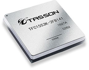
国内首款FC-AE-1553协议ASIC芯片,基于公司具有自主知识产权的总线式拓扑结构,引领产品迈入小型化时代。该芯片功能强大,体积小巧、功耗低,非常适合于功耗、体积要求苛刻的嵌入式系统,能够广泛应用于航空、航天等领域,产品灵活方便,降低开发成本。
TFC1553K芯片支持FC-AE-1553通信协议,可作为FC-AE-1553网络通信节点,实现高速数据接入FC-AE-1553网络的功能。
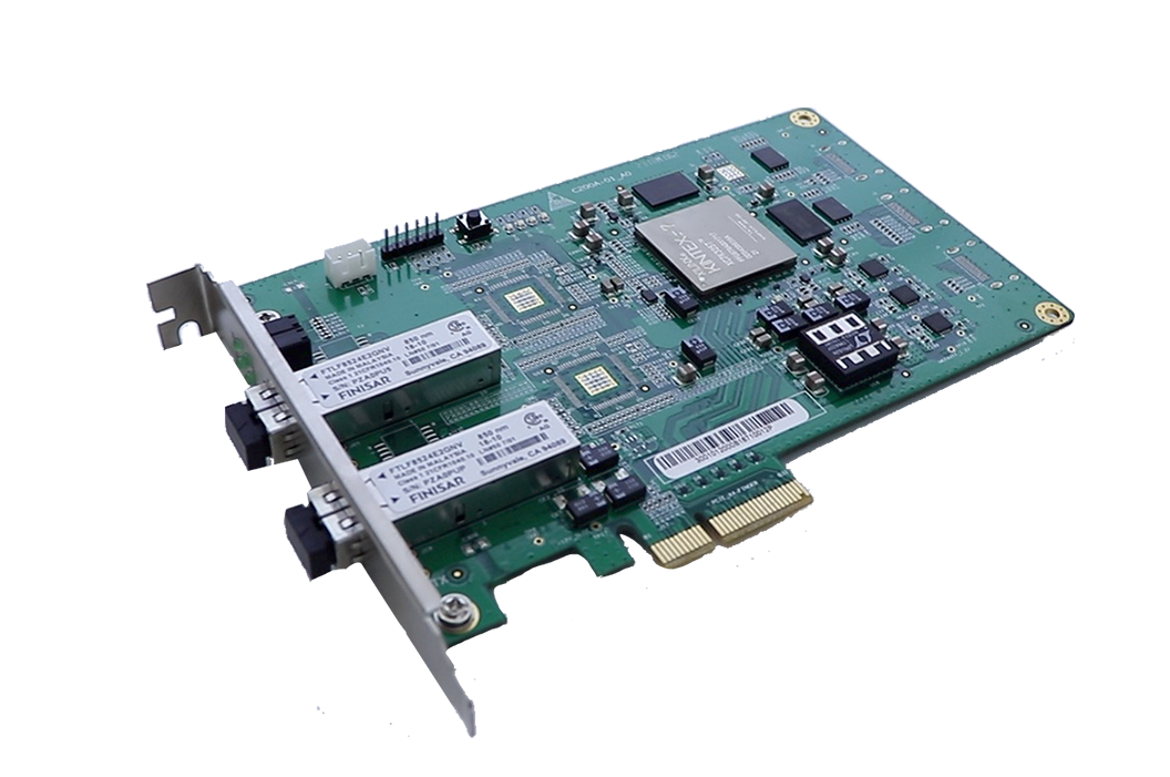
FC-AE-ASM协议光纤通信卡可提供2路FC端口,软件具有友好的人机交互界面,支持协议通信、网络仿真、流量测试、时钟同步和网络管理等功能,便于用户快速搭建FC-AE-ASM网络及测试环境。
本产品是一款8/16口的FC-AE交换板,支持满端口全宽带交换。可提供3U/6U VPX交换板结构,支持风冷/导冷可选。支持根据客户需求定制。
该产品是一款FC-AE-1553总线到MIL-STD-1553B总线的桥接卡。为MIL-STD-1553B接口设备接入FC-AE-1553网络、FC-AE-1553接口设备接入MIL-STD-1553B网络提供支持。
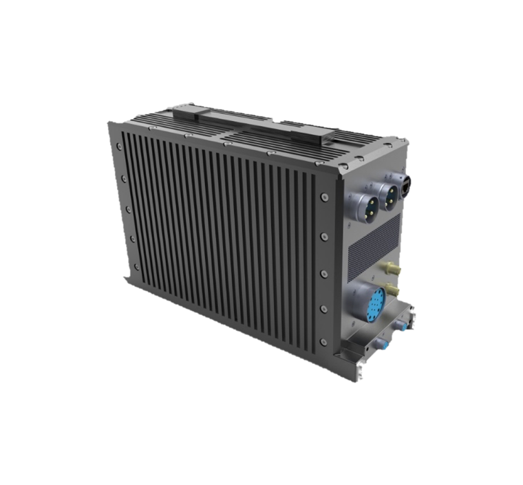
该产品是一款FC-AE-1553总线到MIL-STD-1553B总线的桥接设备。为MIL-STD-1553B接口设备接入FC-AE-1553网络、FC-AE-1553接口设备接入MIL-STD-1553B网络提供支持。
该产品广泛用于FC-AE网络中,能够实现FC总线数据的捕获、存储、分析和统计等功能,可辅助用户研究FC总线通信过程,定位FC总线通信中存在的故障。
故障注入仪用于监控FC链路中的数据,根据触发条件,修改相应的数据帧后发送至链路。用户可用FC故障注入仪搭建网络仿真及测试环境,在特定的数据帧的触发下,修改帧的内容或形式发送回链路,验证用户的设计构想。
DataLink数据链终端支持自组织网络模式,是完全分布式控制部署的高可靠数据链产品。该产品可脱离基础设施,以无中心、自动化的方式动态地形成Ad-Hoc网络,并具有链路自动调节、动态拓扑自动调节的特点。
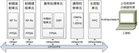
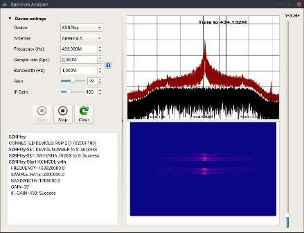
SDR-C/V系列是基于软件无线电的模块化无线系统原理样机开发验证平台,其中,SDR-C系列基于CPCI架构;SDR-V系列基于VPX架构,可升级支持外场加固式设计。
LinkGT地面测试平台是专为数据链与某领域通信设计的综合化地面测试平台,可实现天、空、地、海等不同场景下数据链终端产品无线通信功能、遥测遥控功能或测距测速等功能的验证和测试。
ChE无线信道模拟仪,可在实验室条件下对信道特性进行实时计算与模拟,极大程度地提高通信端机的调试效率并降低对外场测试的依赖,加快产品研发定型速度。
架构方案总览 Architectural solution
实现装备内万物互联,大规模、复杂拓扑、高并发组网方案。
紧贴高可靠应用领域需求,小体积、低功耗、极简总线拓扑光纤组网方案。
具备更优良的适应性,拓扑结构随环境应变,兼顾小体积、低功耗性能的总线拓扑光纤组网方案。
网络利旧,小步快跑,既有同轴电缆网络资源实现千兆网速方案。
解决方案总览 Solution
兼顾指令控制、大数据传输、远距离传输、时间同步的多协议融合舰载电气系统一体化组网解决方案。
采用灵活的光纤一体化网络系统架构,实现空间试验系统组网解决方案。
采用FC-AE-1553技术构建高带宽、低延迟、低功耗、低成本和低重量无人机航电系统网络方案。
新闻动态 News
10月19日,第六届“创客中国”北京市中小企业创新创业大赛暨“创客北京2021”创新创业大赛总结会在京顺利落下帷幕。国科雷速平台-雷速(中国)一站式服务平台凭借坚实的技术实力和自主的创新能力在本次大赛中脱颖而出,获“创客北京2021”企业组二等奖。
12月20日,2020第一届南京大学“励行杯”全球校友创新创业大赛总决赛如期举行,经过现场激烈比拼,国科雷速平台-雷速(中国)一站式服务平台最终荣获一等奖。
11月24日,“直通乌镇”全球互联网大赛总决赛在浙江乌镇举行。经过现场激烈比拼,国科雷速平台-雷速(中国)一站式服务平台最终揽获了总决赛二等奖及最具创新奖两项大奖。
合作伙伴 Partners